Slow R patterns
This document serves as a starting point for code optimizations. It includes possible optimization strategies.
All code here is being benchmarked using the bench package.
For loops vs apply()
Imagine you have a matrix of numbers and you want to compute the row-wise variance. This can be done using a for loop or using the apply function. You will most likely not see any big speed improvements, but the lines of codes can sometimes be considerably be improved.
data <- matrix(rnorm(100000), nrow = 1000)

rowVars <- function(x) {
  x_length <- nrow(x)
  res <- numeric(x_length)
  for (i in seq_len(x_length)) {
    res[i] <- var(x[i, ])
  }
  res
}

bench::mark(
  rowVars = rowVars(data),
  applt = apply(data, 1, var)
)
## # A tibble: 2 x 6
## expression min median `itr/sec` mem_alloc `gc/sec`
## <bch:expr> <bch:tm> <bch:tm> <dbl> <bch:byt> <dbl>
## 1 rowVars 9.09ms 10.8ms 80.6 1.3MB 40.3
## 2 applt 9.21ms 10.3ms 96.9 2.02MB 43.5Apply Sums
If you are about to use apply() with FUN = mean or sum() you might take a look at rowSums(), colsums(), rowMeans(), and colMeans(). They will do the same but faster (NaN and NA are handled slightly differently to tread lightly). the .rowSums() is a faster variant that only works on numeric matrices and does not name the result.
data <- matrix(rnorm(10000), nrow = 100, ncol = 100)

bench::mark(
  apply = apply(data, 1, sum),
  rowSums = rowSums(data),
  .rowSums = .rowSums(data, 100, 100)
) %>% plot()
## Loading required namespace: tidyr
data <- matrix(rnorm(1000000), nrow = 1000, ncol = 1000)

bench::mark(
  apply = apply(data, 1, sum),
  rowSums = rowSums(data),
  .rowSums = .rowSums(data, 1000, 1000)
) %>% plot()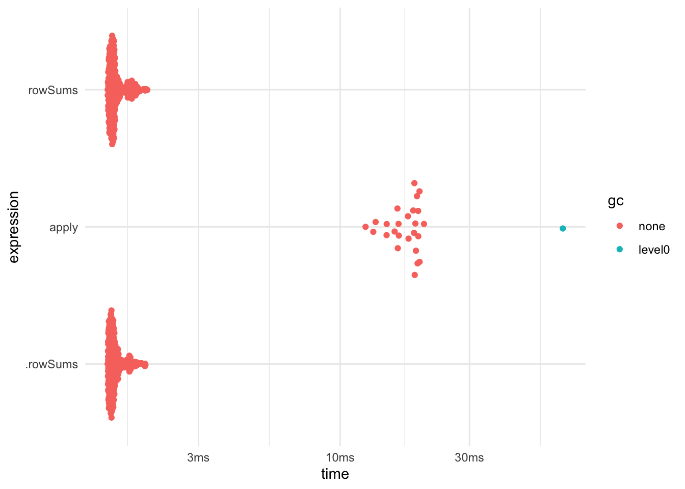

sapply() vs vapply()
bench::mark(
  sapply = sapply(mtcars, sum),
  vapply = vapply(mtcars, sum, FUN.VALUE = numeric(1))
) %>% plot()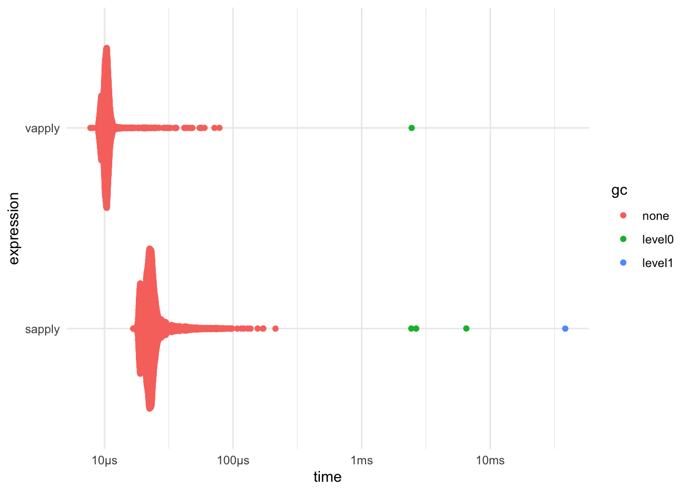
any() function
If you want to see if a vector contains a value, using any(data == 10) can be faster then 10 %in% data. The speed will depend on the length of your vector and how frequent the value is.
bench::press(
  nval = c(10, 100, 1000),
  {
    data <- rpois(nval, 1)
    bench::mark(
      `%in%` = 5 %in% data,
      any = any(data == 5)
    )
  }
) %>% print() %>% plot()
## Running with:
## nval## 1 10## 2 100## 3 1000## # A tibble: 6 x 14
## expression nval min median `itr/sec` mem_alloc `gc/sec` n_itr n_gc
## <bch:expr> <dbl> <bch:tm> <bch:tm> <dbl> <bch:byt> <dbl> <int> <dbl>
## 1 %in% 10 636ns 933ns 979827. 0B 98.0 9999 1
## 2 any 10 376ns 585ns 1420589. 0B 0 10000 0
## 3 %in% 100 1.25µs 1.76µs 457942. 1.27KB 0 10000 0
## 4 any 100 685ns 1.03µs 802915. 448B 0 10000 0
## 5 %in% 1000 3.02µs 7.44µs 156221. 11.81KB 0 10000 0
## 6 any 1000 2.63µs 3.8µs 248829. 3.95KB 0 10000 0
## # … with 5 more variables: total_time <bch:tm>, result <list>, memory <list>,
## # time <list>, gc <list>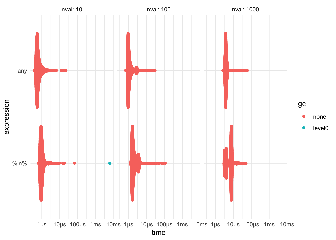
cut() vs findInterval()
Many times when you want to use cut(), to split a vector into bins, it will be faster to replace cut with findInterval as it does less work by not creating a factor.
x <- rnorm(10000)
bench::mark(check = FALSE,
  cut = cut(x, c(-Inf, 0, Inf)),
  findInterval = findInterval(x, c(-Inf, 0, Inf))
) %>%  print() %>% plot()
## # A tibble: 2 x 13
## expression min median `itr/sec` mem_alloc `gc/sec` n_itr n_gc
## <bch:expr> <bch:t> <bch:> <dbl> <bch:byt> <dbl> <int> <dbl>
## 1 cut 486µs 629µs 1531. 273.7KB 2.32 661 1
## 2 findInterval 95.2µs 113µs 8109. 46.3KB 0 4054 0
## # … with 5 more variables: total_time <bch:tm>, result <list>, memory <list>,
## # time <list>, gc <list>
unlist()
unlist() can be sped up by setting use.names = FALSE, this will stop the returned object from being names, saving time.
bench::mark(check = FALSE,
  `use.names = TRUE` = unlist(mtcars),
  `use.names = FALSE` = unlist(mtcars, use.names = FALSE)
)
## # A tibble: 2 x 6
## expression min median `itr/sec` mem_alloc `gc/sec`
## <bch:expr> <bch:tm> <bch:tm> <dbl> <bch:byt> <dbl>
## 1 use.names = TRUE 48.54µs 61.6µs 14582. 5.59KB 0
## 2 use.names = FALSE 2.97µs 3.7µs 204043. 2.8KB 20.4cumulative function and other math group functions
If you have any mathematical calculations you need to have done, it is worth your time to check if they are implemented in R already ?Math.
How many times does Y appear in X
Here we have some object which could be a vector, matrix, or array. we would like to know how many times the number 0 appears.
x_vector <- rpois(10000, 1)

bench::mark(
  table = unname(table(x_vector)["0"]),
  sum = sum(x_vector == 0)
)
## # A tibble: 2 x 6
## expression min median `itr/sec` mem_alloc `gc/sec`
## <bch:expr> <bch:tm> <bch:tm> <dbl> <bch:byt> <dbl>
## 1 table 741.9µs 1.04ms 854. 683KB 2.30
## 2 sum 26.9µs 38.41µs 22216. 39.1KB 2.71table() vs tabulate()
If you need counts of integer-valued vectors, you will gain a big speedup by using the tabulate() function. Notice that tabulate() will ignore non-positive integers, so 0s would not be counted. tabulate will manually place the number of counts of 8 in the 8th place in its output.
## x
##   1   2   3   4   5   6   7   8   9  10
## 86 110 113 88 103 98 95 83 97 127## [1] 86 110 113 88 103 98 95 83 97 127## # A tibble: 2 x 6
## expression min median `itr/sec` mem_alloc `gc/sec`
## <bch:expr> <bch:tm> <bch:tm> <dbl> <bch:byt> <dbl>
## 1 table 136.97µs 154.8µs 6112. 63.3KB 6.61
## 2 tabulate 4.08µs 4.9µs 195094. 0B 0Using pipes
The use of the pipe operator %>% can make your code more readable, but it will also result in (slightly) slower code. If speed is very important you might want to reconsider using pipes. This will be a trade-off between readability and speed.
library(magrittr)
x <- rpois(1000, 1)

bench::mark(
  `pipe` = x %>% identity(),
  `no pipe` = identity(x)
) %>%
  print() %>%
  plot()
## # A tibble: 2 x 13
## expression min median `itr/sec` mem_alloc `gc/sec` n_itr n_gc total_time
## <bch:expr> <bch:t> <bch:t> <dbl> <bch:byt> <dbl> <int> <dbl> <bch:tm>
## 1 pipe 47.3µs 59.4µs 16067. 280B 14.7 7664 7 477.01ms
## 2 no pipe 245ns 435ns 1608263. 0B 0 10000 0 6.22ms
## # … with 4 more variables: result <list>, memory <list>, time <list>, gc <list>
Summing weights
If you need to calculate the Matrix cross product then it is usually faster to use crossprod() then use the t(x) %*% y
x <- matrix(rnorm(1000), ncol = 1)
w <- matrix(rnorm(10000), ncol = 10)

bench::mark(
  `%*%` = t(x) %*% w,
  `crossprod` = crossprod(x, w)
)
## # A tibble: 2 x 6
## expression min median `itr/sec` mem_alloc `gc/sec`
## <bch:expr> <bch:tm> <bch:tm> <dbl> <bch:byt> <dbl>
## 1 %*% 19µs 25.5µs 36084. 7.86KB 3.61
## 2 crossprod 14.9µs 18.9µs 48820. 2.23KB 0pmax() and pmin()
pmin is a nice shorthand, but you can gain some speed with some rewriting.
## # A tibble: 2 x 6
##   expression      min   median `itr/sec` mem_alloc `gc/sec`
##   <bch:expr> <bch:tm> <bch:tm>     <dbl> <bch:byt>    <dbl>
## 1 pmin         8.79µs  11.38µs    72721.    7.86KB     14.5
## 2 rewrite      3.65µs   4.71µs   192391.   17.13KB      0
lm()
If you are doing linear regression, and you already have the data as matrices you can benefit greatly from using the .lm.fit() function. This function will not do any checking for you. Just the calculations.
y <- mtcars$mpg

x <- as.matrix(mtcars[, c("disp", "cyl")])

bench::mark(check = FALSE,
  lm = lm(mpg ~ disp + cyl - 1, mtcars),
  .lm.fit = .lm.fit(x, y)
)
## # A tibble: 2 x 6
## expression min median `itr/sec` mem_alloc `gc/sec`
## <bch:expr> <bch:tm> <bch:tm> <dbl> <bch:byt> <dbl>
## 1 lm 535.85µs 616.72µs 1546. 5.36KB 13.9
## 2 .lm.fit 2.74µs 3.54µs 260781. 3.99KB 0using : for creating sequences
Creating a sequence from 1 to n.
n <- 100000

bench::mark(
  seq = seq(1, n),
  seq.int = seq.int(1, n),
  `:` = 1:n,
  seq_len = seq_len(n)
)
## # A tibble: 4 x 6
## expression min median `itr/sec` mem_alloc `gc/sec`
## <bch:expr> <bch:tm> <bch:tm> <dbl> <bch:byt> <dbl>
## 1 seq 3.86µs 5.72µs 156455. 0B 15.6
## 2 seq.int 308ns 417ns 2304088. 0B 0
## 3 : 152ns 207ns 4498116. 0B 0
## 4 seq_len 125ns 178ns 4898761. 0B 0Not only is seq_len() faster, but it is also safer as it works well when n = 0.
## [1] 1 0## integer(0)