The aphylo R package implements estimation and data imputation methods for Functional Annotations in Phylogenetic Trees. The core function consists of the log-likelihood computation of observing a given phylogenetic tree with functional annotation on its leaves and the probabilities associated to gain and loss of function, including probabilities of experimental misclassification. The log-likelihood is computed using peeling algorithms, which required developing and implementing efficient algorithms for re-coding and preparing phylogenetic tree data to be used with the package. Finally, aphylo works smoothly with popular tools for analysis of phylogenetic data such as ape R package, “Analyses of Phylogenetics and Evolution.”
The package is under MIT License and is developed by the Computing and Software Cores of the Biostatistics Division’s NIH Project Grant (P01) at the Department of Preventive Medicine at the University of Southern California.
Citation
citation(package="aphylo")When using aphylo, please cite the following paper:
Vega Yon GG, Thomas DC, Morrison J, Mi H, Thomas PD, et al. (2021)
Bayesian parameter estimation for automatic annotation of gene
functions using observational data and phylogenetic trees. PLOS
Computational Biology 17(2): e1007948.
https://doi.org/10.1371/journal.pcbi.1007948
And the actual R package:
Vega Yon G (????). _Statistical Inference of Annotated Phylogenetic
Trees_. R package version 0.3-5,
<https://github.com/USCBiostats/aphylo>.
To see these entries in BibTeX format, use 'print(<citation>,
bibtex=TRUE)', 'toBibtex(.)', or set
'options(citation.bibtex.max=999)'.Install
This package depends on another on-development R package, the fmcmc. So first, you need to install it:
devtools::install_github("USCbiostats/fmcmc")Then you can install the aphylo package
devtools::install_github("USCbiostats/aphylo")Reading data
# This datasets are included in the package
data("fakeexperiment")
data("faketree")

head(fakeexperiment)
head(faketree)
O <- new_aphylo(
  tip.annotation = fakeexperiment[,2:3],
  tree           = as.phylo(faketree)
)

O
Phylogenetic tree with 4 tips and 3 internal nodes.
Tip labels:
1, 2, 3, 4
Node labels:
5, 6, 7
Rooted; no branch length.
Tip (leafs) annotations:
f1 f2
1 0 0
2 0 1
3 1 0
4 1 1
Internal node annotations:
f1 f2
5 9 9
6 9 9
7 9 9
as.phylo(O)Phylogenetic tree with 4 tips and 3 internal nodes.
Tip labels:
1, 2, 3, 4
Node labels:
5, 6, 7
Rooted; no branch length.
# We can visualize it
plot(O)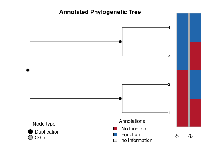
plot_logLik(O)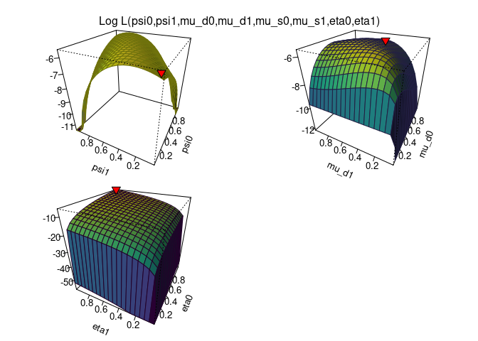
Simulating annotated trees
set.seed(198)
dat <- raphylo(
  50,
  P    = 1,
  psi  = c(0.05, 0.05),
  mu_d = c(0.8, 0.3),
  mu_s = c(0.1, 0.1),
  Pi   = .4
  )

dat
Phylogenetic tree with 50 tips and 49 internal nodes.
Tip labels:
1, 2, 3, 4, 5, 6, ...
Node labels:
51, 52, 53, 54, 55, 56, ...
Rooted; no branch length.
Tip (leafs) annotations:
fun0000
1 1
2 0
3 0
4 1
5 0
6 0
...(44 obs. omitted)...
Internal node annotations:
fun0000
1 1
2 1
3 1
4 1
5 1
6 0
...(43 obs. omitted)...Estimation
# Using L-BFGS-B (MLE) to get an initial guess
ans0 <- aphylo_mle(dat ~ psi + mu_d + Pi + eta)


# MCMC method
ans2 <- aphylo_mcmc(
  dat ~ mu_d + mu_s + Pi,
  prior   = bprior(c(9, 1, 1, 1, 5), c(1, 9, 9, 9, 5)),
control = list(nsteps=5e3, burnin=500, thin=10, nchains=2))Warning: While using multiple chains, a single initial point has been passed
via `initial`: c(0.9, 0.5, 0.1, 0.05, 0.5). The values will be recycled.
Ideally you would want to start each chain from different locations.
Convergence has been reached with 5500 steps. Gelman-Rubin's R: 1.0097. (500 final count of samples).
ans2ESTIMATION OF ANNOTATED PHYLOGENETIC TREE
Call: aphylo_mcmc(model = dat ~ mu_d + mu_s + Pi, priors = bprior(c(9,
1, 1, 1, 5), c(1, 9, 9, 9, 5)), control = list(nsteps = 5000,
burnin = 500, thin = 10, nchains = 2))
LogLik (unnormalized): -20.1333
Method used: mcmc (5500 steps)
# of Leafs: 50
# of Functions 1
# of Trees: 1
Estimate Std. Err.
mu_d0 0.9107 0.0797
mu_d1 0.1648 0.0800
mu_s0 0.1157 0.0735
mu_s1 0.1001 0.0442
Pi 0.5329 0.1450
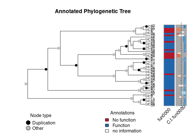
plot(
  ans2,
  nsample = 200,
  loo     = TRUE,
  ncores  = 2L
  )
# MCMC Diagnostics with coda
library(coda)
gelman.diag(ans2$hist)
Potential scale reduction factors:
Point est. Upper C.I.
mu_d0 1.01 1.05
mu_d1 1.00 1.00
mu_s0 1.00 1.02
mu_s1 1.01 1.02
Pi 1.00 1.00
Multivariate psrf
1.01
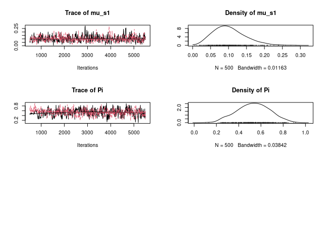
plot(ans2$hist)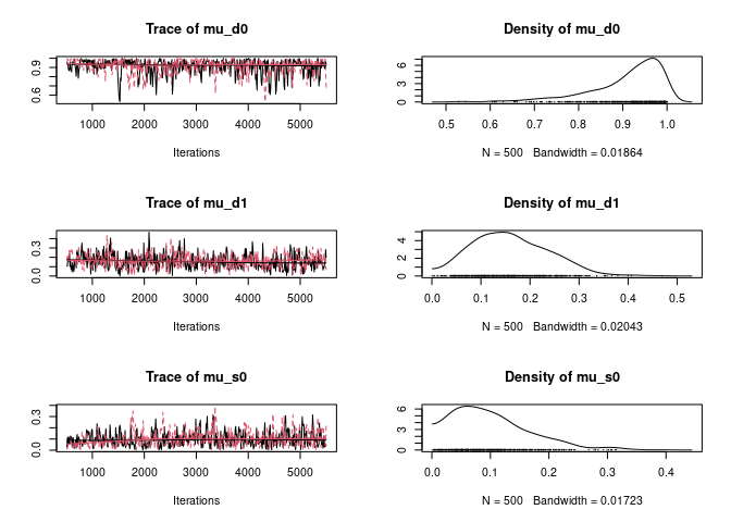
Prediction
pred <- prediction_score(ans2, loo = TRUE)
pred
Prediction score (H0: Observed = Random)
N obs. : 99
alpha(0, 1) : 0.26, 0.74
Observed : 0.71
Random : 0.62
P(<t) : 0.1121
--------------------------------------------------------------------------------
Values scaled to range between 0 and 1, 1 being best.
Significance levels: *** p < .01, ** p < .05, * p < .10
AUC 0.79.
MAE 0.29.
plot(pred)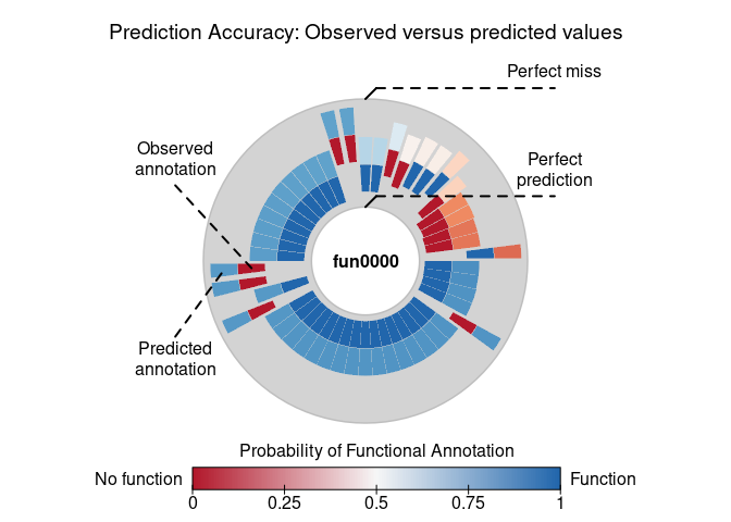
Misc
During the development process, we decided to allow the user to choose what ‘tree-reader’ function he would use, particularly between using either the rncl R package or ape. For such, we created a short benchmark that compares both functions here.