Objects of class aphylo_estimates — aphylo

The model fitting of annotated phylogenetic trees can be done using either MLE via aphylo_mle() or MCMC via aphylo_mcmc(). This section describes the object of class aphylo_estimates that these functions generate and the post estimation methods/functions that can be used.

# S3 method for class 'aphylo_estimates'
print(x, ...)

# S3 method for class 'aphylo_estimates'
coef(object, ...)

# S3 method for class 'aphylo_estimates'
vcov(object, ...)

# S3 method for class 'aphylo_estimates'
plot(
  x,
  y = NULL,
  which.tree = 1L,
  ids = list(1:Ntip(x)[which.tree]),
  loo = TRUE,
  nsamples = 1L,
  ncores = 1L,
  centiles = c(0.025, 0.5, 0.975),
  cl = NULL,
  ...
)

Arguments

x, object: Depending of the method, an object of class aphylo_estimates.
...: Further arguments passed to the corresponding method.
y: Ignored.
which.tree: Integer scalar. Which tree to plot.
ids, nsamples, ncores, centiles, cl: passed to predict.aphylo_estimates()
loo: Logical scalar. When loo = TRUE, predictions are preformed similar to what a leave-one-out cross-validation scheme would be done (see predict.aphylo_estimates).

Value

Objects of class aphylo_estimates are a list withh the following elements:

par: A numeric vector of length 5 with the solution.
hist: A numeric matrix of size counts*5 with the solution path (length 2 if used optim as the intermediate steps are not available to the user). In the case of aphylo_mcmc, hist is an object of class coda::mcmc.list().
ll: A numeric scalar with the value of fun(par, dat). The value of the log likelihood.
counts: Integer scalar number of steps/batch performed.
convergence: Integer scalar. Equal to 0 if optim converged. See optim.
message: Character scalar. See optim.
fun: A function (the objective function).
priors: If specified, the function priors passed to the method.
dat: The data dat provided to the function.
par0: A numeric vector of length 5 with the initial parameters.
method: Character scalar with the name of the method used.
varcovar: A matrix of size 5*5. The estimated covariance matrix.

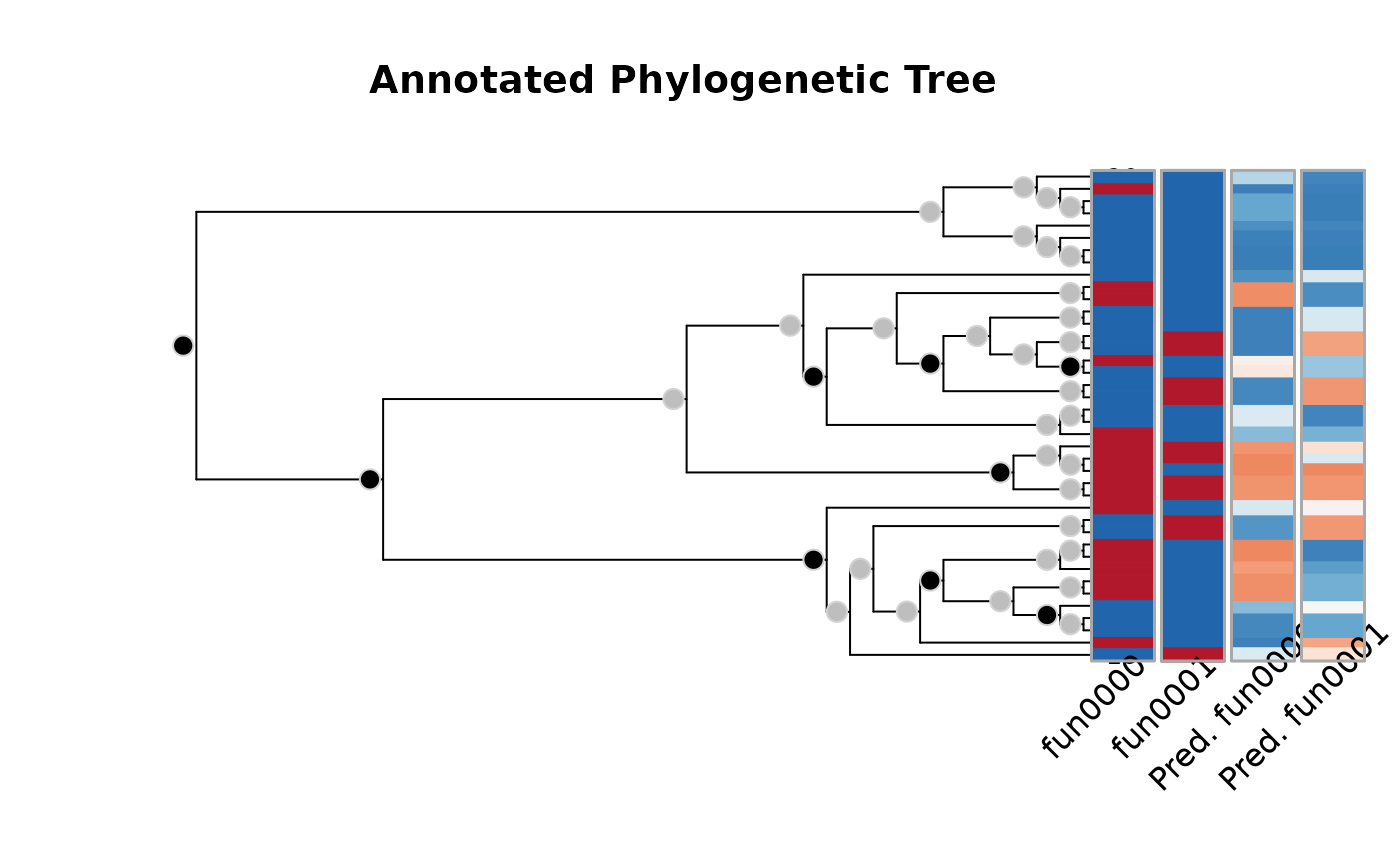
The plot method for aphylo_estimates returns the selected tree (which.tree) with predicted annotations, also of class aphylo.

Details

The plot method for the object of class aphylo_estimates plots the original tree with the predicted annotations.

Examples

set.seed(7881)
atree <- raphylo(40, P = 2)
res   <- aphylo_mcmc(atree ~ mu_d + mu_s + Pi)
#> Warning: While using multiple chains, a single initial point has been passed via `initial`: c(0.9, 0.5, 0.1, 0.05, 0.5). The values will be recycled. Ideally you would want to start each chain from different locations.
#> Convergence has been reached with 10000 steps. Gelman-Rubin's R: 1.0233. (500 final count of samples).

print(res)
#> 
#> ESTIMATION OF ANNOTATED PHYLOGENETIC TREE
#> 
#>  Call: aphylo_mcmc(model = atree ~ mu_d + mu_s + Pi)
#>  LogLik: -37.7731 
#>  Method used: mcmc (10000 steps)
#>  # of Leafs: 40
#>  # of Functions 2
#>  # of Trees: 1
#> 
#>          Estimate  Std. Err.
#>  mu_d0   0.8392    0.1475
#>  mu_d1   0.5985    0.1571
#>  mu_s0   0.1515    0.0702
#>  mu_s1   0.0544    0.0320
#>  Pi      0.5076    0.2971
#> 
coef(res)
#>      mu_d0      mu_d1      mu_s0      mu_s1         Pi 
#> 0.83921480 0.59853604 0.15148002 0.05436977 0.50762014 
vcov(res)
#>              mu_d0         mu_d1         mu_s0         mu_s1            Pi
#> mu_d0  0.021761402  0.0064170422 -0.0013305666 -0.0000281820  0.0035925925
#> mu_d1  0.006417042  0.0246873308  0.0027730753 -0.0007584415 -0.0038793095
#> mu_s0 -0.001330567  0.0027730753  0.0049245626 -0.0003601076  0.0014041022
#> mu_s1 -0.000028182 -0.0007584415 -0.0003601076  0.0010221978 -0.0001894985
#> Pi     0.003592593 -0.0038793095  0.0014041022 -0.0001894985  0.0882936562
plot(res)