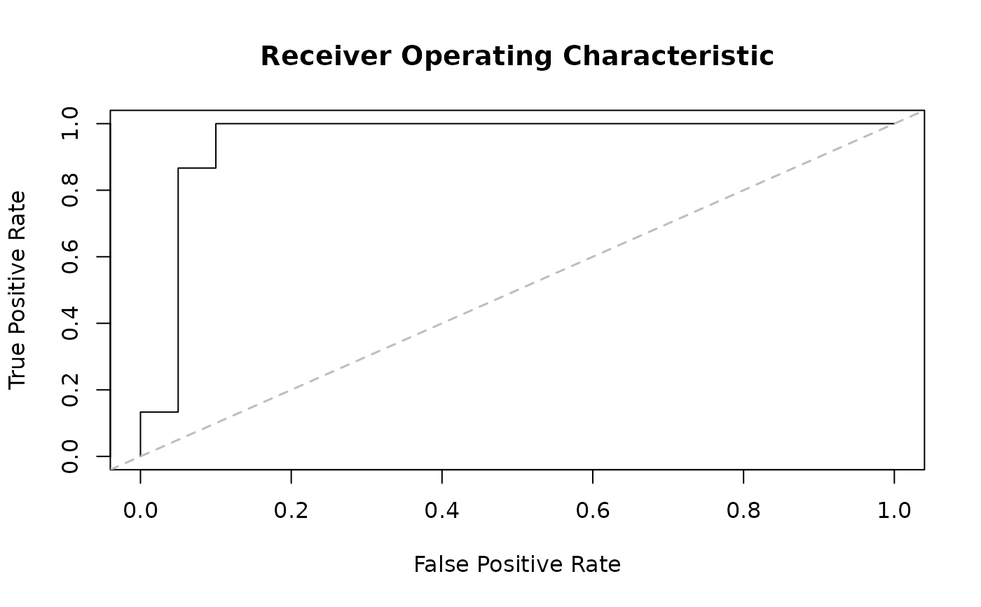
The AUC values are computed by approximation using the area of the polygons formed under the ROC curve.
Arguments
- pred
A numeric vector with the predictions of the model. Values must range between 0 and 1.
- labels
An integer vector with the labels (truth). Values should be either 0 or 1.
- nc
Integer. Number of cutoffs to use for computing the rates and AUC.
- nine_na
Logical. When
TRUE, 9 is treated asNA.- x
An object of class
aphylo_auc.- ...
Further arguments passed to the method.
- y
Ignored.
Value
A list:
tprA vector of lengthncwith the True Positive Rates.tnrA vector of lengthncwith the True Negative Rates.fprA vector of lengthncwith the False Positive Rates.fnrA vector of lengthncwith the False Negative Rates.aucA numeric value. Area Under the Curve.cutoffsA vector of lengthncwith the cutoffs used.
Examples
set.seed(8381)
x   <- rdrop_annotations(raphylo(50), .3)
ans <- aphylo_mcmc(x ~ mu_d + mu_s + Pi)
#> Warning: While using multiple chains, a single initial point has been passed via `initial`: c(0.9, 0.5, 0.1, 0.05, 0.5). The values will be recycled. Ideally you would want to start each chain from different locations.
#> Convergence has been reached with 10000 steps. Gelman-Rubin's R: 1.0144. (500 final count of samples).
ans_auc <- auc(predict(ans, loo = TRUE), x[,1,drop=TRUE])
print(ans_auc)
#> Number of observations     : 35
#> Area Under The Curve (AUC) : 0.95
#> Rates can be accessed via the $ operator.
plot(ans_auc)
