Week 8: Efficiency and High Performance Computing

PM 566: Introduction to Health Data Science

George G. Vega Yon and Kelly Street

Part I: Efficiency

Why does it matter?

Often, we will want to do the same task (or similar tasks) many times with only slight differences.

Some tasks are very “computationally expensive” meaning they require a lot of time or other resources to run.

In these cases, computational efficiency can be very important. It can mean the difference between a job that takes two hours to run as opposed two weeks!

Efficiency: Loops

We’ve seen various examples of loops so far in this class.

Classic examples that are common to most programming languages include for and while loops.

Other types of loops are more specific to R, such as the various *apply functions (apply, sapply, lapply, etc.).

Knowing when to use a loop and when not to is a critical concern in computational efficiency.

Example: Square Roots

Let’s say we want to take the square roots of the numbers 1 to 10,000. We could achieve this in a number of different ways.

Here, we use a for loop:

forLoopRoots <- function(n){
  roots <- rep(NA, n)
  for(i in 1:n){
    roots[i] <- sqrt(i)
  }
  return(roots)
}

head(forLoopRoots(10000))

[1] 1.000000 1.414214 1.732051 2.000000 2.236068 2.449490

Example: Square Roots (cont. 1)

Here, we’ll use sapply:

SapplyRoots <- function(n){
  roots <- sapply(1:n, sqrt)
  return(roots)
}

head(SapplyRoots(10000))

[1] 1.000000 1.414214 1.732051 2.000000 2.236068 2.449490

Example: Square Roots (cont. 2)

How fast are these methods? Let’s use the microbenchmark package to find out!

library(microbenchmark)
microbenchmark(forLoopRoots(10000), SapplyRoots(10000))

Unit: microseconds
                expr     min       lq      mean   median        uq      max
 forLoopRoots(10000) 186.386  202.007  208.8872  209.264  214.9015  235.709
  SapplyRoots(10000) 987.731 1075.553 1190.6945 1099.600 1158.5575 4815.163
 neval
   100
   100

Example: Square Roots (cont. 3)

But do we really need a loop for this job? Here, we’ll use vectorization to perform all the calculations “at once.”

VectorizedRoots <- function(n){
  sqrt(1:n)
}

head(VectorizedRoots(10000))

[1] 1.000000 1.414214 1.732051 2.000000 2.236068 2.449490

Example: Square Roots (cont. 4)

That’s a lot faster!

library(microbenchmark)
microbenchmark(forLoopRoots(10000), VectorizedRoots(10000))

Unit: microseconds
                   expr     min       lq      mean   median       uq     max
    forLoopRoots(10000) 188.313 191.8595 205.54858 203.2165 211.8265 340.341
 VectorizedRoots(10000)   8.036  14.3090  20.37167  14.8010  15.6620 503.234
 neval
   100
   100

Anytime that you can use vectorized computation, you should! It will (almost) always save you a lot of computation time!

Use pre-made functions

Let’s say there’s a relatively simple operation you want to perform. You know how to write the code for it, but you’re pretty sure there’s also a built-in function that performs the same task. Which should you use?

Generally speaking, you should aim to write as little code as possible. Built-in functions (especially in the base package) are highly optimized and likely to run much faster than manual implementations.

Example: Repeated elements

Let’s say we have a long vector and we want to find all of the repeated elements.

set.seed(1)
vec <- sample(letters, 100, replace = TRUE)
vec

  [1] "y" "d" "g" "a" "b" "w" "k" "n" "r" "s" "a" "u" "u" "j" "v" "n" "j" "g"
 [19] "i" "o" "u" "e" "i" "y" "n" "e" "e" "b" "j" "y" "l" "o" "a" "t" "c" "f"
 [37] "j" "j" "f" "o" "t" "t" "z" "l" "y" "w" "f" "y" "h" "l" "y" "w" "x" "f"
 [55] "z" "g" "s" "j" "f" "x" "n" "b" "m" "r" "v" "n" "f" "a" "s" "s" "h" "f"
 [73] "w" "l" "f" "h" "g" "k" "q" "d" "m" "h" "y" "p" "y" "w" "n" "t" "g" "m"
 [91] "v" "l" "p" "a" "m" "u" "f" "q" "i" "g"

Example: Repeated elements (cont. 1)

We can achieve this with two nested loops:

method1 <- function(x){
  # first element cannot be a duplicate
  out <- sapply(2:length(x), function(i){
    matches <- sapply(1:(i-1), function(i2){
      x[i2] == x[i]
    })
    return(any(matches))
  })
  out <- c(FALSE, out)
  return(out)
}

vec[1:11]

 [1] "y" "d" "g" "a" "b" "w" "k" "n" "r" "s" "a"

method1(vec)[1:11]

 [1] FALSE FALSE FALSE FALSE FALSE FALSE FALSE FALSE FALSE FALSE  TRUE

Example: Repeated elements (cont. 2)

Or slightly faster with a loop and vectorized comparison:

method2 <- function(x){
  # first element cannot be a duplicate
  out <- sapply(2:length(x), function(i){
    return(any(x[1:(i-1)] == x[i]))
  })
  out <- c(FALSE, out)
  return(out)
}

method2(vec)[1:11]

 [1] FALSE FALSE FALSE FALSE FALSE FALSE FALSE FALSE FALSE FALSE  TRUE

microbenchmark(method1(vec), method2(vec))

Unit: microseconds
         expr      min        lq      mean   median        uq      max neval
 method1(vec) 2046.679 2152.0900 2330.1743 2205.082 2308.0335 4164.165   100
 method2(vec)   73.021   78.5355  108.9657   81.877   87.4735 1590.718   100

Example: Repeated elements (cont. 3)

But the real speed-up comes when we use the base function duplicated:

method3 <- function(x){
  duplicated(x)
}

method3(vec)[1:11]

 [1] FALSE FALSE FALSE FALSE FALSE FALSE FALSE FALSE FALSE FALSE  TRUE

microbenchmark(method2(vec), method3(vec))

Unit: microseconds
         expr    min      lq     mean median     uq     max neval
 method2(vec) 76.998 80.6675 84.63015 82.328 85.608 113.693   100
 method3(vec)  1.353  1.5785  5.76050  1.722  1.927 397.864   100

Part II: High Performance Computing

What is HPC?

High Performance Computing (HPC) can relate to any of the following:

Parallel computing, i.e. using multiple resources (could be threads, cores, nodes, etc.) simultaneously to complete a task.
Big data working with large datasets (in/out-of-memory).

We will mostly focus on parallel computing.

Serial computation

Here we are using a single core. The function is applied one element at a time, leaving the other 3 cores without usage.

Parallel computation

In this more intelligent way of computation, we are taking full advantage of our computer by using all 4 cores at the same time. This will reduce computation time which, in the case of complicated/long calculations, can be an important speed gain.

Parallel computing: Hardware

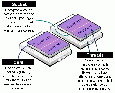
When it comes to parallel computing, there are several ways (levels) in which we can speed up our analysis. From the bottom up:

Thread level SIMD instructions: Most modern processors support some level of what is called vectorization, this is, applying a single (same) instruction to streams of data. For example: adding vector A and B.
Hyper-Threading Technology (HTT): Intel’s hyper-threading generates a virtual partition of a single core (processor) which, while not equivalent to having multiple physical threads, does speed things up.
Multi-core processor: Most modern CPUs (Central Processing Unit) have two or more physical cores. A typical laptop computer has about 8 cores.
General-Purpose Computing on Graphics Processing Unit (GP-GPU): While modern CPUs have multiple cores, GPUs can hold thousands of cores. Designed for image processing, there’s an increasing use of GPUs as an alternative to CPUs for scientific computing.

Parallel computing: Hardware (cont.)

High-Performance Computing Cluster (HPC): A collection of computing nodes that are interconnected using a fast Ethernet network.
Grid Computing: A collection of loosely interconnected machines that may or may not be in the same physical place, for example: HTCondor clusters.

Parallel computing: CPU components

Taxonomy of CPUs (Downloaded from https://slurm.schedmd.com/mc_support.html)

Ask yourself these questions before jumping into HPC!

Parallel computing in R

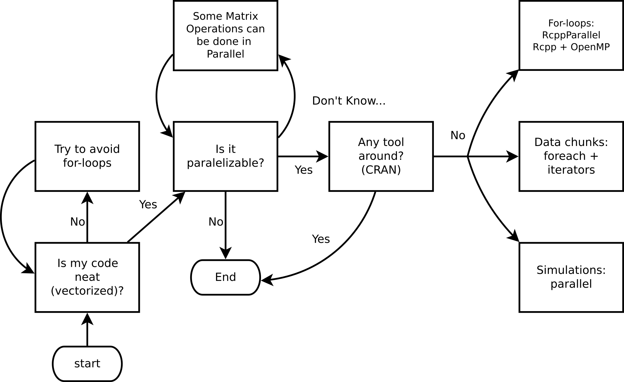
While there are several alternatives (just take a look at the High-Performance Computing Task View), we’ll focus on the following R-packages for explicit parallelism

Some examples:

parallel: R package that provides ‘[s]upport for parallel computation, including random-number generation’.

foreach: R package for ‘general iteration over elements’ in parallel fashion.

future: ‘[A] lightweight and unified Future API for sequential and parallel processing of R expression via futures.’ (won’t cover here)

Implicit parallelism, on the other hand, are out-of-the-box tools that allow the programmer not to worry about parallelization, e.g. such as gpuR for Matrix manipulation using GPU, tensorflow

And there’s also a more advanced set of options

Rcpp + OpenMP: Rcpp is an R package for integrating R with C++, and OpenMP is a library for high-level parallelism for C/C++ and Fortran.

A ton of other type of resources, notably the tools for working with batch schedulers such as Slurm, HTCondor, etc.

The `parallel` package

Based on the snow and multicore R Packages.
Explicit parallelism.
Simple yet powerful idea: Parallel computing as multiple R sessions.
Clusters can be made of both local and remote sessions
Multiple types of cluster: PSOCK, Fork, MPI, etc.

Parallel workflow

(Usually) We do the following:

Create a PSOCK/FORK (or other) cluster using makePSOCKCluster/makeForkCluster (or simply makeCluster)
Copy/prepare each R session (if you are using a PSOCK cluster):
1. Copy objects with clusterExport
2. Set a seed with clusterSetRNGStream
Do your call:
1. Pass expressions with clusterEvalQ
2. Run a parallelized loop with parApply, parLapply, etc.
Stop the cluster with clusterStop

Ex 1: Hello world!

# 1. CREATING A CLUSTER
library(parallel)
cl <- makeCluster(4)    
x  <- 20

# 2. PREPARING THE CLUSTER
clusterSetRNGStream(cl, 123) # Equivalent to `set.seed(123)` (not necessary for this example)
clusterExport(cl, "x")

# 3. DO YOUR CALL
clusterEvalQ(cl, {
  paste0("Hello from process #", Sys.getpid(), ". I see x and it is equal to ", x)
})

[[1]]
[1] "Hello from process #30604. I see x and it is equal to 20"

[[2]]
[1] "Hello from process #30603. I see x and it is equal to 20"

[[3]]
[1] "Hello from process #30606. I see x and it is equal to 20"

[[4]]
[1] "Hello from process #30605. I see x and it is equal to 20"

# 4. STOP THE CLUSTER
stopCluster(cl)

Ex 1: Hello world! (redux)

Multi-core versions of the *apply functions are simpler, but may not work on Windows machines.

# 1. SETUP
library(parallel)
x  <- 20

# 2. DO YOUR CALL
mclapply(1:4, function(i){
    paste0("Hello from process #", Sys.getpid(), ". I see x and it is equal to ", x)
}, mc.cores = 4)

[[1]]
[1] "Hello from process #30658. I see x and it is equal to 20"

[[2]]
[1] "Hello from process #30659. I see x and it is equal to 20"

[[3]]
[1] "Hello from process #30660. I see x and it is equal to 20"

[[4]]
[1] "Hello from process #30661. I see x and it is equal to 20"

Ex 2: Parallel regressions

Problem: Run multiple regressions on a very wide dataset. We need to fit the following model:

\[ y = X_i\beta_i + \varepsilon,\quad \varepsilon\sim N(0, \sigma^2_i),\quad\forall i \]

[1] 500 999

         x001        x002       x003       x004      x005
1  0.61827227  1.72847041 -1.4810695 -0.2471871 1.4776281
2  0.96777456 -0.19358426 -0.8176465  0.6356714 0.7292221
3 -0.04303734 -0.06692844  0.9048826 -1.9277964 2.2947675
4  0.84237608 -1.13685605 -1.8559158  0.4687967 0.9881953
5 -1.91921443  1.83865873  0.5937039 -0.1410556 0.6507415
6  0.59146153  0.81743419  0.3348553 -1.8771819 0.8181764

 num [1:500] -0.8188 -0.5438 1.0209 0.0467 -0.4501 ...

Ex 2: Parallel regressions (cont. 1)

Serial solution: Use apply (basic loop) to solve it

#
#
#
#
ans <- apply(
  X = X,
  MARGIN = 2,
  FUN = function(x) coef(lm(y ~ x))
)

ans[,1:5]

                   x001        x002        x003        x004        x005
(Intercept) -0.03449819 -0.03339681 -0.03728140 -0.03644192 -0.03717344
x           -0.06082548  0.02748265 -0.01327855 -0.08012361 -0.04067826

Ex 2: Parallel regressions (cont. 2)

Parallel solution: Use parApply

library(parallel)
cl <- makeCluster(4L)
clusterExport(cl, "y")
ans <- parApply(
  cl = cl,
  X = X,
  MARGIN = 2,
  FUN = function(x) coef(lm(y ~ x))
)
 
ans[,1:5]

                   x001        x002        x003        x004        x005
(Intercept) -0.03449819 -0.03339681 -0.03728140 -0.03644192 -0.03717344
x           -0.06082548  0.02748265 -0.01327855 -0.08012361 -0.04067826

Ex 2: Parallel regressions (cont. 3)

Are we going any faster?

microbenchmark::microbenchmark(
  parallel = parApply(
    cl = cl,
    X = X, MARGIN = 2,
    FUN = function(x) coef(lm(y ~ x))
  ),
  serial = apply(
    X = X, MARGIN = 2,
    FUN = function(x) coef(lm(y ~ x))
  ), unit="relative"
)

Unit: relative
     expr      min       lq     mean   median       uq      max neval
 parallel 1.000000 1.000000 1.000000 1.000000 1.000000 1.000000   100
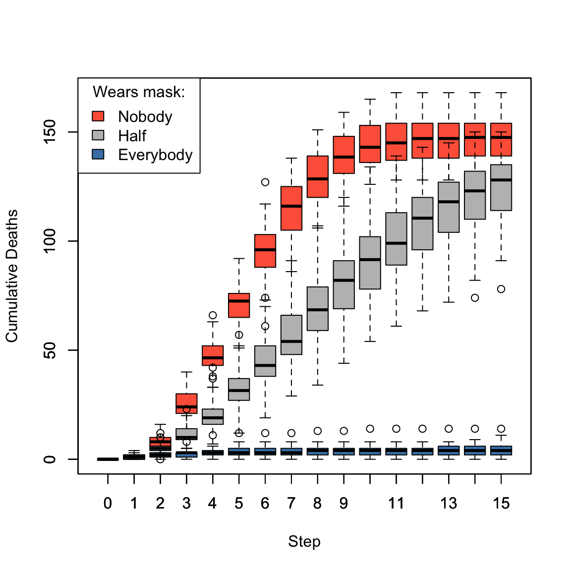
   serial 2.603318 2.623148 2.589386 2.613118 2.616343 2.258219   100

Part II: Extended Example

Extended Example: SARS-CoV2 simulation

An altered version of Conway’s game of life

People live on a grid, each individual having 8 neighbors.
A healthy individual (A) interacting with a sick neighbor (B) has the following probabilities of contracting the disease:
1. 100% if neither wears a mask.
2. 50% if only A wears a mask.
3. 20% if only B wears a mask.
4. 5% if both wear masks.
Infected individuals may die with probability 10%.

We want to illustrate the importance of wearing face masks. We are going to simulate a system with 2,500 (50 x 50) individuals, 1,000 times so we can analyze: (a) contagion curve, (b) death curve.

More models like this: The SIRD model (Susceptible-Infected-Recovered-Deceased)

Conway’s Game of Masks

Download the program here.

# source("~/Downloads/sars-cov2.R", echo=FALSE)
source("img/sars-cov2.R", echo = FALSE)

# Looking at some constants
probs_sick # Sick individual's probabilities

 deceased  infected recovered 
      0.1       0.4       0.5

probs_susc # Probabilities of i getting the disease

               j doesn't wear j wears
i doesn't wear            0.9    0.20
i wears                   0.5    0.05

First look: What does the simulation look like?

   susceptible infected recovered deceased
0         1440      160         0        0
1         1265      234        85       16
2         1064      307       190       39
3          876      321       334       69
4          717      287       499       97
15         430        1       990      179
16         429        2       990      179
17         429        0       992      179
18         429        0       992      179
19         429        0       992      179

First look: What does the simulation look like? (contd’)

# Location of who wears the facemask. This step is only for plotting
wears <- which(one$wears, arr.ind = TRUE) - 1
wears <- wears/(one$nr) * (1 + 1/one$nr)

# Initializing the animation
fig   <- magick::image_device(600, 600, res = 96/2, pointsize = 24)
for (i in 1:one$current_step) {
  
  # Plot
  image(
    one$temporal[,,i], col=c("gray", "tomato", "steelblue","black"),
    main = paste("Time", i - 1L, "of", one$nsteps),
    zlim = c(1,4)
    )
  points(wears, col="white", pch=20, cex=1.5)
  legend(
    "topright",
    col = c("gray", "tomato", "steelblue","black", "black"),
    legend = c(names(codes), "wears a mask"),
    pch = c(rep(15, 4), 21)
  )
}

# Finalizing plot and writing the animation
dev.off()
animation <- magick::image_animate(fig, fps = 2)
magick::image_write(animation, "covid1.gif")

Cumulative number of deceased as a function of whether none, half, or all individuals wear a face mask.

Speed things up: Timing under the serial implementation

We will use the function system.time to measure how much time it takes to complete 20 simulations in serial versus parallel fashion using 4 cores.

Speed things up: Parallel a Forking Cluster

Alternative 1: If you are using Unix-like system (Ubuntu, OSX, etc.), you can take advantage of process forking, and thus, parallel’s mclapply function:

Speed things up: Parallel with a Socket Cluster

Alternative 2: Regardless of the operating system, we can use a Socket cluster, which is simply a group of fresh R sessions that listen to the parent/main/mother session.

# Step 2: Prepare the cluster
# We could either export all the needed variables
parallel::clusterExport(
  cl,
  c("calc_stats", "codes", "dat", "get_neighbors", "init", "probs_sick",
    "probs_susc", "simulate_covid", "update_status", "update_status_all"
    )
  )

Or simply run the simulation script in the other sessions:

# Step 2 (alt): Prepare the cluster
parallel::clusterEvalQ(cl, source("img/sars-cov2.R"))
parallel::clusterSetRNGStream(cl, 123) # Make sure it is reproducible!

Bonus: Checking what are the processes running on the system

(pids <- c(
  master    = Sys.getpid(),
  offspring = unlist(parallel::clusterEvalQ(cl, Sys.getpid()))
  ))
#      master offspring1 offspring2 
#     14810      15998      16012

Speed things up: Parallel with a Socket Cluster (cont’d)

Using two threads/processes, you can obtain the following speedup

   user  system elapsed 
  6.049   0.038   6.090

   user  system elapsed 
  0.000   0.000   3.292

   user  system elapsed 
  0.000   0.010   3.309

Part III: Cloud Computing

Cloud Computing (a.k.a. on-demand computing)

HPC clusters, super-computers, etc. need not be bought… you can rent:

These services provide more than just computing (storage, data analysis, etc.). But for computing and storage, there are other free resources, e.g.:

The Extreme Science and Engineering Discovery Environment (XSEDE)

There are many ways to run R in the cloud

At USC:

Center for Advanced Research Computing (CARC). USC users can request hundreds of cores (literally).

Running R in:

Google Cloud: https://cloud.google.com/solutions/running-r-at-scale
Amazon Web Services: https://aws.amazon.com/blogs/big-data/running-r-on-aws/
Microsoft Azure: https://docs.microsoft.com/en-us/azure/architecture/data-guide/technology-choices/r-developers-guide

Submitting jobs

A key feature of cloud services: interact via command line.
You will need to be familiar with Rscript and R CMD BATCH.
Which is better? It depends on the application.

Submitting jobs (examples)

Imagine we have the following R script (download here):

library(data.table)
set.seed(1231)
dat <- data.table(y = rnorm(1e3), x = sample.int(5, 1e3, TRUE))
dat[,mean(y), by = x]

R CMD BATCH

This will run a non-interactive R session and put all the output (stdout and stderr) to the file dummy.Rout.

R CMD BATCH --vanilla dummy.R dummy.Rout &

Rscript

This will also execute R in the background, with the difference that the output dummy.Rout will not capture stderr (messages, warnings and errors from R).

Rscript --vanilla dummy.R > dummy.Rout &

The & at the end makes sure the job is submitted and does not wait for it to end.

Rscript

The R script can be executed as a program directly, if you specify where the Rscript program lives.

The following example works on Unix. This is an R script named since_born.R (download here)

#!/usr/bin/Rscript
args <- tail(commandArgs(), 0)
message(Sys.Date() - as.Date(args), " days since you were born.")

This R script can be executed in various ways…

Rscript as a program

For this we would need to change it to an executable. In unix you can use the chmod command: chmod +x since_born.R. This allows us to do the following:

Rscript in a bash script (most common)

In the case of running jobs on a cluster or something similar, we usually need to have a bash script. In our case, we have a file named since_born_bash.sh that calls Rscript (download here)

#!/bin/bash
Rscript since_born.R 1988-03-02

Which we would execute like this:

Fatal error: cannot open file 'since_born.R': No such file or directory

Summary

Parallel computing can speed things up.
It’s not always needed… make sure that you are taking advantage of vectorization.
Most loops can be parallelized (“embarrassingly parallel computing”).
In R, explicit parallelism can be achieved using the parallel package:
1. Load the package and create a cluster: library(parallel), parallel::makeCluster()
2. Setup the environment: parallel::clusterExport(), parallel::clusterSetRNGStream()
3. Make the call: parallel::clusterEvalQ(), parallel::parLapply()
4. Stop the cluster: parallel::stopCluster()
Regardless of the Cloud computing service we are using, we will be using either R CMD BATCH or Rscript to submit jobs.

Session info

R version 4.5.0 (2025-04-11)
Platform: aarch64-apple-darwin20
Running under: macOS Sequoia 15.6.1

Matrix products: default
BLAS:   /Library/Frameworks/R.framework/Versions/4.5-arm64/Resources/lib/libRblas.0.dylib 
LAPACK: /Library/Frameworks/R.framework/Versions/4.5-arm64/Resources/lib/libRlapack.dylib;  LAPACK version 3.12.1

locale:
[1] en_US.UTF-8/en_US.UTF-8/en_US.UTF-8/C/en_US.UTF-8/en_US.UTF-8

time zone: America/Los_Angeles
tzcode source: internal

attached base packages:
[1] parallel  stats     graphics  grDevices utils     datasets  methods  
[8] base     

other attached packages:
[1] microbenchmark_1.5.0 scales_1.4.0         RColorBrewer_1.1-3  

loaded via a namespace (and not attached):
 [1] digest_0.6.37     R6_2.6.1          fastmap_1.2.0     xfun_0.52        
 [5] farver_2.1.2      glue_1.8.0        knitr_1.50        htmltools_0.5.8.1
 [9] rmarkdown_2.29    lifecycle_1.0.4   cli_3.6.5         compiler_4.5.0   
[13] rstudioapi_0.17.1 tools_4.5.0       evaluate_1.0.4    yaml_2.3.10      
[17] jsonlite_2.0.0    rlang_1.1.6

(Bonus) `Rcpp`: R & C++

The Fibonacci series

\[ Fib(n) = \left\{\begin{array}{ll} n & \mbox{if }n \leq 1 \\ Fib(n-1) + Fib(n - 2) & \mbox{otherwise} \end{array}\right. \]

Rcpp: Hello world! v1

The following C++ file, called fib.cpp

Can be compiled within R using Rcpp::sourceCpp("fib.cpp"). This exports the function back into R:

[1] 1 1 2 3 5

Rcpp: Hello world! v2 (with function overloading)

Rcpp data types are mapped directly to R data types, e.g. vectors of integers in R can be used as IntegerVector in Rcpp.

Back in R

[1] 1 1 2 3 5

RcppArmadillo and OpenMP

Friendlier than RcppParallel… at least for ‘I-use-Rcpp-but-don’t-actually-know-much-about-C++’ users (like myself!).
Must run only ‘Thread-safe’ calls, so calling R within parallel blocks can cause problems (almost all the time).
Use arma objects, e.g. arma::mat, arma::vec, etc. Or, if you are used to them std::vector objects as these are thread safe.
Pseudo-Random Number Generation is not very straight forward… But C++11 has a nice set of functions that can be used together with OpenMP
Need to think about how processors work, cache memory, etc. Otherwise you could get into trouble… if your code is slower when run in parallel, then you probably are facing false sharing
If R crashes… try running R with a debugger (see Section 4.3 in Writing R extensions):
```
~$ R --debugger=valgrind
```

RcppArmadillo and OpenMP workflow

Add the following to your C++ source code to use OpenMP, and tell Rcpp that you need to include that in the compiler:
```
#include <omp.h>
// [[Rcpp::plugins(openmp)]]
```
Tell the compiler that you’ll be running a block in parallel with openmp
```
#pragma omp [directives] [options]
{
  ...your neat parallel code...
}
```
You’ll need to specify how OMP should handle the data:
- shared: Default, all threads access the same copy.
- private: Each thread has its own copy (although not initialized).
- firstprivate Each thread has its own copy initialized.
- lastprivate Each thread has its own copy. The last value is the one stored in the main program.
Setting default(none) is a good practice.
Compile!

Ex 3: RcppArmadillo + OpenMP

Computing the distance matrix (see ?dist)

#include <Rcpp.h>
#include <omp.h>
#include <RcppArmadillo.h>
// [[Rcpp::depends(RcppArmadillo)]]
// [[Rcpp::plugins(openmp)]]
using namespace Rcpp;

// [[Rcpp::export]]
arma::mat dist_par(const arma::mat & X, int cores = 1) {
  
  // Some constants and the result
  int N = (int) X.n_rows; int K = (int) X.n_cols;
  arma::mat D(N,N,arma::fill::zeros);
  
  omp_set_num_threads(cores); // Setting the cores
  
#pragma omp parallel for shared(D, N, K, X) default(none)
  for (int i=0; i<N; ++i)
    for (int j=0; j<i; ++j) {
      for (int k=0; k<K; k++) 
        D.at(i,j) += pow(X.at(i,k) - X.at(j,k), 2.0);
      
      // Computing square root
      D.at(i,j) = sqrt(D.at(i,j)); D.at(j,i) = D.at(i,j);
    }
      
  // My nice distance matrix
  return D;
}

set.seed(1231)
K <- 1000
n <- 500
x <- matrix(rnorm(n*K), ncol=K)

# Benchmarking!
microbenchmark::microbenchmark(
  dist(x),                 # stats::dist
  dist_par(x, cores = 1),  # 1 core
  dist_par(x, cores = 2),  # 2 cores
  times = 10, unit="relative"
)

Resources

For more, checkout the CRAN Task View on HPC

Simulating $\pi$

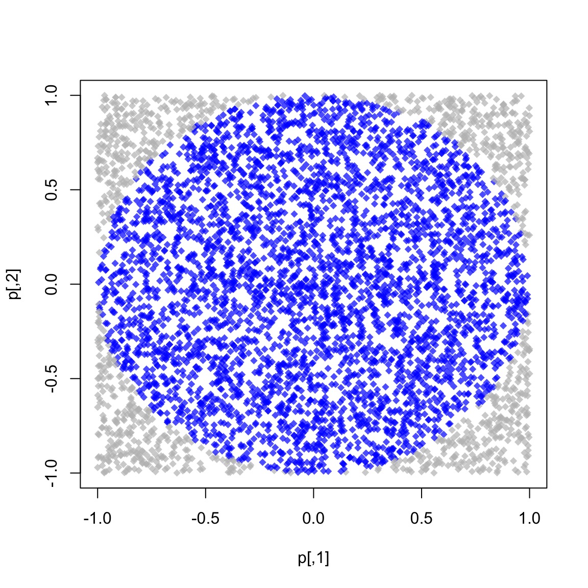
We know that $\pi = \frac{A}{r^2}$. We approximate it by randomly adding points $x$ to a square of size 2 centered at the origin.
So, we approximate $\pi$ as $\Pr\{\|x\| \leq 1\}\times 2^2$

The R code to do this

pisim <- function(i, nsim) {  # Notice we don't use the -i-
  # Random points
  ans  <- matrix(runif(nsim*2), ncol=2)
  
  # Distance to the origin
  ans  <- sqrt(rowSums(ans^2))
  
  # Estimated pi
  (sum(ans <= 1)*4)/nsim
}

library(parallel)
# Setup
cl <- makeCluster(4L)
clusterSetRNGStream(cl, 123)

# Number of simulations we want each time to run
nsim <- 1e5

# We need to make -nsim- and -pisim- available to the
# cluster
clusterExport(cl, c("nsim", "pisim"))

# Benchmarking: parSapply and sapply will run this simulation
# a hundred times each, so at the end we have 1e5*100 points
# to approximate pi
microbenchmark::microbenchmark(
  parallel = parSapply(cl, 1:100, pisim, nsim=nsim),
  serial   = sapply(1:100, pisim, nsim=nsim), times = 1, unit="relative"
)

Unit: relative
     expr      min       lq     mean   median       uq      max neval
 parallel 1.000000 1.000000 1.000000 1.000000 1.000000 1.000000     1
   serial 2.220003 2.220003 2.220003 2.220003 2.220003 2.220003     1

(Bonus) Overview of HPC

Using Flynn’s classical taxonomy, we can classify parallel computing according to the following two dimensions:

Type of instruction: Single vs Multiple
Data stream: Single vs Multiple

(Bonus) Parallel computing: Software

Implicit parallelization:

tensorflow: Machine learning framework
pqR: Branched version of R.
Microsoft R: Microsoft’s R private version (based on Revolution Analytics’ R version).
data.table (R package): Data wrangling using multiple cores.
caret (R package): A meta package, has various implementations using parallel computing.

Explicit parallelization (DIY):

CUDA (C/C++ library): Programming with GP-GPUs.
Open MP (C/C++ library): Multi-core programming (CPUs).
Open MPI (C/C++ library): Large scale programming with multi-node systems.
Threading Building Blocks (C/C++ library): Intel’s parallel computing library.
Kokkos (C++ library): A hardware-agnostic programming framework for HPC applications.
parallel (R package): R’s built-in parallel computing package
future (R package): Framework for parallelzing R.
RcppParallel (R C++ API wrapper): Header and templates for building Rcpp+multi-threaded programs.
julia (programming language): High-performing, has a framework for parallel computing as well.