Schedule

Lecture 11 (Last week):

• Creating interactive graphs with plotly for R package and tables with DataTable

Lecture 12 (Today):

• Create a website using R Markdown and GitHub Pages (like this!)
• Share interactive plots on the website
• Note: Assignment due Friday (hpc and sql)

11/23 Thanksgiving Holiday

11/30 Lecture 13 Final Project Workshop

• Note: Assignment due Dec 2 (interactive viz I and II)

Interactive visualization: Topics covered

Last week:

• Interactive plots (plotly)

• Interactive maps (plotly, Leaflet)

• Interactive tables (DT)

This week:

We will build static websites using R Markdown and GitHub Pages. We will learn how to render text, code, visuals, and interactive visuals (e.g. with plotly, leaflet, DT, etc.) on the website.

Building websites in R Markdown with GitHub Pages

To understand how websites are built in R Markdown, we first must understand a bit about how R Markdown documents are rendered to produce HTML output.

It is not essential to understand all the inner workings of this process to be able to create a website. However, it is important to understand which component is responsible for what since this will make it easier to target appropriate help files when you need them!

What does R Markdown require to render files?

R Markdown combines several different processes together to create documents. In doing so it requires the use of a few essential ingredients (software and packages):

• R Markdown: A markup language for creating .Rmd files that you have used.

• rmarkdown: An R package for processesing and converting .Rmd files into a number of different formats.

• knitr: An R package for transforming a mixture of R code and text in a .Rmd file into a .md file by executing the code and 'knitting' the results back into the document.

• Pandoc: A document converter. It is designed to convert plain text files from one markup language (including .Rmd files) into many output formats. It is a command line software with no GUI. Although is separate from R, it comes bundled with R Studio because rmarkdown relies on it for document conversion.

A note on formatting: word indicates an R package, while word indicates inline code or file name/format. word() indicates a function. Software programs (e.g. R Markdown and Pandoc) are not given a special formatting.

What happens when we render R Markdown files?

The basic workflow structure for an R Markdown document is shown below, highlighting the steps (arrows) and the intermediate files that are created before producing the output.

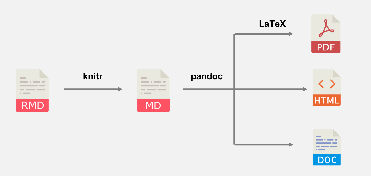
Rendering R Markdown documents with rmarkdown consists of converting .Rmd to .md with knitr, and then .md to our desired output with Pandoc.

What happens when we render R Markdown files? (cont'd)

The workflow in more detail is as follows:

1. The .Rmd document is written. It is the original format of the document. It contains a combination of YAML (metadata in the header), text, and code chunks. The YAML header specifies document properties and rendering instructions (like html_document for HTML output)

2. The knit() function in knitr is used to execute all code embedded within the .Rmd file, and prepare the code output to be displayed within the output document. knitr handles the execution and translation of all code in the file. All these results are converted into the correct markup language and contained within a temporary .md file.

3. The .md file is processed by Pandoc. It takes any parameters specified within the YAML frontmatter of the document (e.g., title, author, and date) to convert the document to the output format specified in the output parameter (in our case: html_document for HTML output)

4. The whole process is implemented by R Markdown (the software) via the function from the built-in rmarkdown (package): rmarkdown::render()

Along the way, we add structure and style. A wide range of tools helps us in this process. For creating HTML output, some of these include Cascading Style Sheets (CSS) for adding style (e.g., fonts, colors, spacing) to Web documents, raw HTML code, and Pandoc templates.

YAML metadata

YAML = Yet Another Markup Language YAML Ain't Markup Language

It is a data-oriented language structure used as the input format for diverse software application. It is not a markup language (which includes indicators or "markup" which direct processing) but a serialization language. Serialization is the process of converting an object into a format that can be transmitted or stored, by converting the object series of bits. This series of bits is then read later to reconstruct the object.

YAML metadata

A typical YAML header looks like this, and contains basic metadata about the document and rendering instructions:

---
title: My R Markdown Website
author: Abigail Horn
output: html_document
---

The YAML metadata affects the code, content, and the output. It is processed during many stages of the rendering process by rmarkdown, knitr, and Pandoc:

• The title and author fields are processed by Pandoc to set the values of template variables

• The output field is used by rmarkdown to apply the output format function rmarkdown::html_document() in the rendering process. For creating a website we will need to pass additional arguments to the format that we are specifying in output.

We will come back to specify the YAML metadata necessary for setting up a website.

Beyond Pandoc

Note that not all R Markdown documents are eventually compiled through Pandoc. The intermediate .md file could be compiled by other Markdown renderers, including:

• The xaringan package passes the .md output to a JavaScript library, which renders the Markdown content in the web browser. All slides for this course have been produced using this package!

• The blogdown package supports the .Rmarkdown document format, which is knitted to .md, and this Markdown document is usually rendered to HTML by an external site generator. Using blogdown is another way to create a website out of R Markdown (but today we will be focusing on creating websites using rmarkdown and Pandoc)

Summary: What happens when we render R Markdown files?

In short: rmarkdown::render() = knitr::knit() + Pandoc

The YAML metadata in the R Markdown file dictates the process and how the output is produced.

Website basics

The most common components of a web page are HTML, CSS, and JavaScript. HTML is relatively simple to learn, but CSS and JavaScript can be much more complicated, depending on how much you want to learn and what you want to do with them.

You don't need to know much of HTML, CSS, or JavaScript to develop a website using R Markdown. If you want to tweak the appearance of your website, you must have some basic knowledge of web development.

HTML basics

HTML = Hyper Text Markup Language. HTML is a standard markup language (not programming language) that provides the primary structure of most websites.

HTML defines the basic structure of a web page. HTML work on the look of the website without the interactive effects and all. HTML pages are static which means the content cannot be changed.

All elements in HTML are represented by tags. Most HTML tags appear in pairs, with an opening tag and a closing tag, and content is placed between the opening and closing tags, e.g., <span style="background-color: #B9BFFF">This is highlighted text</span> --> This is highlighted text.

There are a few exceptions, such as the <img> tag, which can be closed by a slash / in the opening tag, e.g., <img src="foo.png" />. You can specify attributes of an element in the opening tag using the syntax name=value (a few attributes do not require value).

Basically an HTML document consists a head section and body section. You can specify the metadata and include assets like CSS files in the head section.

You can use View -> Developer -> Source to see HTML source code.

Helpful HTML

Font size and color <font size="3" color="red">Text here!</font>

Columns <div class="col2"> and </div>

Centered text <center>**Here the text is centered. Here are good resources:**</center>

Small image right-aligned <div align="right"><img src="images/Rmd_cheatsheet.png" width="150px"></div>

Large image centered: <center><img src="images/Rmd_cheatsheet.png" width="500px"></center>

CSS basics

CSS = Cascading Stylesheets (CSS). It is a markup language is used to describe the look and formatting of documents written in HTML. it is responsible for the visual style of your site, responsible for components including:

• color palettes,
• images,
• layouts/margins
• fonts

as well as onteractive components like

• dropdown menus
• buttons, and
• forms

There are 3 ways to define styles:

• in-line with HTML
• placing a style section in your HTML document
• define the CSS in an external file that is then referenced as a link in your HTML (most flexible)

JavaScript

JavaScript is an advanced programming language (unlike HTML and CSS, which do not contain any programming logic) that makes web pages more interactive and dynamic. JavaScript simply adds dynamic content to websites to make them look good. JavaScript can be embedded inside HTML.

An effective way to learn it is through the JavaScript console in the Developer Tools of your web browser because you can interactively type code in the console and execute it, which feels similar to executing R code in the R console (e.g., in RStudio). You may open any web page in your web browser, then open the JavaScript console, and try the code below on any web page:

document.body.style.background = 'orange';

Which should turn the background orange, unless the page has already defined background colors for certain elements.

To effectively use JavaScript, you have to learn both the basic syntax of JavaScript and how to select elements on a page before you can manipulate them.

Learn more on the blogdown website To effectively use JavaScript, you have to learn both the basic syntax of JavaScript and how to select elements on a page before you can manipulate them.

Website basics: learning more

The best way to learn about what goes into web development: use "Developer Tools", e.g. View -> Developer in Google Chrome. Or right click and "inspect".

A brief intro to HTML, CSS, and JavaScript is provided in the blogdown book

You can also learn more at w3schools or course StackOverflow!

Building a website using rmarkdown

Background: Static vs. dynamic websites

A dynamic site relies on a server-side language to do certain computing and sends potentially different content depending on different conditions. A common language is PHP, and a typical example of a dynamic site is a web forum. For example, each user has a profile page, but typically this does not mean the server has stored a different HTML profile page for every single user. Instead, the server will fetch the user data from a database, and render the profile page dynamically.

A static site consists of static files such as HTML, CSS, JavaScript, images, etc., and the web server sends exactly the same content to the web browser no matter who visits the web pages. There is no dynamic computing on the server when a page is requested. It is just one folder of static files.

Creating websites through rmarkdown

rmarkdown has a built-in static site generator, which we will be using today. It uses Bootstrap CSS styles and themes (which you can choose from).

There are many existing static site generators, including Hugo, Jekyll, and Hexo, etc. These provide many site themes, templates, and features, but are more complex than rmarkdown's built-in generator.

rmarkdown's site generator is a good option if:

• You are familiar with generating single-page HTML output from R Markdown
• You want to build a simple website with a few pages
• It suffices to use a flat directory of .Rmd files
• You don't require features such as forums or RSS feeds

Creating websites through rmarkdown

We can render collections of R Markdown documents as a website using the rmarkdown::render_site() function

The RStudio IDE (version 1.0 or higher) also includes integrated support for developing R Markdown websites through the Build toolbar. These make use of an RStudio Project tied to your website's directory.

In lab, we will use the RStudio IDE and command line to build our websites, and deploy them on GitHub pages. We will focus on both local and remote setup.

The focus of the remaining lecture component will be to overview the pieces needed to create a website, and provide some background on different features to be aware of.

Overview

There are two main steps for creating a personal website that will be hosted on GitHub:

• Create website through local setup
• Deploy website through GitHub setup

Overview: Local Setup

1. Create a project directory and an R Project file (.Rproj)
2. Create a _site.yml and index.Rmd file in your new directory
3. Add additional page content if desired through other .Rmd files
4. Edit these files to create content and manage layout (and knit to view)
5. Add a style sheet (CSS) if desired
6. Build website
   • Build tab > Build Website or
   • in the console: rmarkdown::render_site() This creates the output: index.html

Let's break this down, foucusing on the essential content of the website.

Essential elements

The minimum requirement for any R Markdown website is that it have an index.Rmd file as well as a _site.yml file.

To start with, let's walk through a very simple example, a website that includes two pages (Home and About) and a navigation bar to switch between them.

A simple example

First, we need a configuration file _site.yml:

name: "my-website"
navbar:
  title: "My Website"
  left:
    - text: "Home"
      href: index.html
    - text: "About"
      href: about.html

A simple example (cont'd)

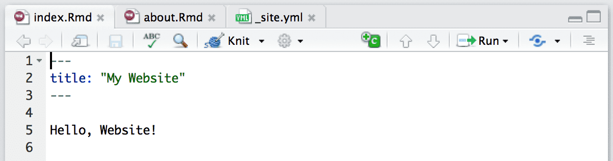
Then two Rmd files, index.Rmd:

---
title: "My Website"
---
Hello, Website!

and about.Rmd:

---
title: "About This Website"
---
More about this website.

Common elements

Now let's talk in a bit more detail about the essential _site.yml, the index.Rmd, and other non-essential common elements.

Typically when creating a website, there are various common elements you want to include on all pages (e.g., output options, CSS styles, header and footer elements, etc.)

Common elements: _site.yml

A more detailed _site.yml could look like this:

name: "my-website"
output_dir: "."
navbar:
  title: "My Website"
  left:
    - icon: fa-home
      href: index.html
    - text: "About"
      href: about.html
  right:
    - text: "External website"
    - href: www.google.com
output:
  html_document:
    theme: cosmo
    highlight: textmate
    include:
      after_body: footer.html
    css: styles.css

Common elements: _site.yml

• The name field provides a suggested URL path for your website when it is published (by default this is just the name of the directory containing the site).

• The output_dir field indicates which directory to copy site content into ("_site" is the default if none is specified). It can be "." to keep all content within the root website directory alongside the source code.

• The output element within our _site.yml file defines shared output options for all R Markdown documents within a site. Note that individual documents can also include their own output options, which will be merged with the common options at render time.

  • As part of our common output options, we have specified an HTML footer (via the include: after-body: option) and a CSS stylesheet. You can also include HTML before the body or in the document's <head>

• In addition to whatever common options you define in the _site.yml, there are two output options that are automatically set when rendering a site:

  • The self_contained option is set FALSE
  • The lib_dir option is set to site_libs.

These options are set so that dependent files (e.g. HTML widget libraries) are shared across all documents within the site rather than redundantly embedded within each document.

_site.yml: navbar

The navbar element of _site.yml can be used to define a common navigation bar for your website. You can include internal and external links on the navigation bar as well as drop-down menus for sites with a large number of pages.

Some capabilities of navigation bars:

• You can use the type field to choose between the default and inverse navigation bar styles (each theme includes distinct colors for "default" and "inverse" navigation bars).

• You can align navigational items either to the left or to the right.

• You can include both internal and external links on the navigation bar.

• You can use icons on the navigation bar. Icons from three different icon sets are available.

  • Font Awesome
  • Ionicons
  • Bootstrap Glyphicons

When referring to an icon, you should use its full name including the icon set prefix (e.g., fa-github, ion-social-twitter, and glyphicon-time).

Common elements: other

• Include a footer: footer.html:

  <p>Copyright &copy; 2016 Skynet, Inc. All rights reserved.</p>

• Style sheets: styles.css

  blockquote {
    font-style: italic
  }

Rendering and building the site

As you work on the individual pages of your website, you can render them using the Knit button just as you do with conventional standalone R Markdown documents

Knitting an individual page will only render and preview that page, not the other pages in the website.

To render all of the pages in the website, you use the Build pane, which calls rmarkdown::render_site() to build and then preview the entire site

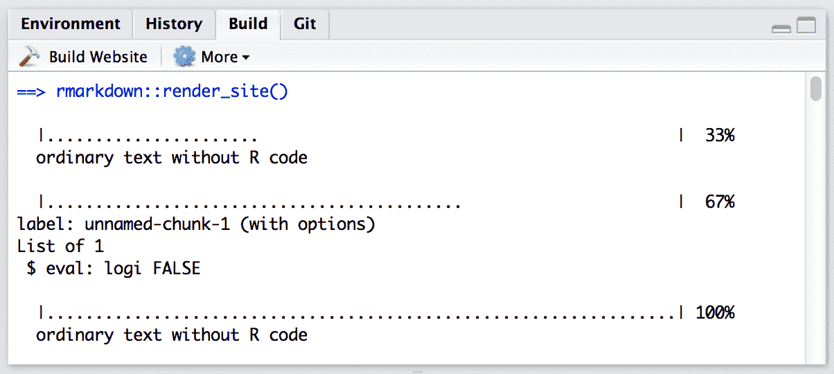
Build an entire website in RStudio.

Rendering and building the site (cont'd)

RStudio supports "live preview" of changes that you make to supporting files within your website (e.g., CSS, JavaScript, .Rmd partials, R scripts, and YAML config files).

Changes to CSS and JavaScript files always result in a refresh of the currently active page preview. Changes to other files (e.g., shared scripts and configuration files) trigger a rebuild of the active page (this behavior can be disabled via the options dialog available from the Build pane).

Note that only the active page is rebuilt, so once you are happy with the results of rendering you should make sure to rebuild the entire site from the Build pane to ensure that all pages inherit your changes.

In other words, you need to re-build the website to integrate any new changes to one page.

Rendering and building the site: command line

Or from command line: you can call the render_site() function directly from within the website directory. Pass no arguments to render the entire site or a single file in order to render just that file:

# render the entire site
rmarkdown::render_site()
# render a single file only
rmarkdown::render_site("about.Rmd")

If you execute the rmarkdown::render_site() function from within the directory containing the website, the following will occur:

• All of the *.Rmd and *.md files in the root website directory will be rendered into HTML. Note, however, that Markdown files beginning with _ are not rendered (this is a convention to designate files that are to be included by top level Rmd documents as child documents).

• The generated HTML files and any supporting files (e.g., CSS and JavaScript) are copied into an output directory (_site by default).

• The HTML files within the _site directory are now ready to deploy as a standalone static website.

Note: The include and exclude fields of _site.yml can be used to override this default behavior

Helpful features

R Markdown website themes

R Markdown makes styling easy for you. The HTML output of R Markdown includes the Bootstrap framework. Bootstrap has multiple themes we can choose from.

We can change the website’s theme in _site.yml. Explore themes here

Valid themes include “default”, “cerulean”, “journal”, “flatly”, “readable”, “spacelab”, “united”, “cosmo”, “lumen”, “paper”, “sandstone”, “simplex”, and “yeti”.

R scripts

If you have R code that you would like to share across multiple R Markdown documents within your site, you can create an R script (e.g., utils.R) and source it within your Rmd files. For example:

```{r}
source("utils.R")
```

Adding interactive content

R Markdown includes many facilities for generation of HTML content from R objects, including:

• The conversion of standard R output types (e.g., ggplot2 objects) within code chunks done automatically by knitr

• A variety of ways to generate HTML tables, including the knitr::kable() function and other packages such as kableExtra

• A large number of available HTML widgets (e.g., plotly objects) that provide rich JavaScript data visualizations.

As a result, for many R Markdown websites you will not need to worry about generating HTML output at all (since it is created automatically).

Saving interactive plots as HTML widgets

If you are having issues with embedding interactive plots, you can use the package widgetframe to save HTML files via an HTML iframe. This is convenient not only for re-using a widget in various parent documents, but also for preventing any JavaScript and CSS in the parent document from negatively impacting how the widget renders

The widgetframe package automates the saving of widgetframe packages into and has options for controling where, how, and if external dependencies are stored on the file system when using it inside a knitr/rmarkdown document. widgetframe is designed to be used in .Rmd documents which will eventually be knitted to an HTML or a derived format. Use the default options and embed files like this:

```{r}
library(widgetframe)
test.widget <- plot_ly()
widgetframe::frameWidget(test.widget, width = '75%')
```

widgetframe will take care of embedding the supporting HTML widget libraries in a folder together.

Adding dynamic content

To add something dynamic and always changing with external input (like a comment box), you can incorporate an outside commenting system like Disqus. Disqus is a third-party service that provides comment and community capabilities to websites via JavaScript.

knitr caching

If your website is time consuming to render, you may want to enable knitr's caching during the development of the site, so that you can more rapidly preview. To enable caching for an individual chunk, just add the cache = TRUE chunk option:

```{r, cache = TRUE}
data <- longComputation()
```

To enable caching for an entire document, add cache = TRUE to the global chunk option defaults:

```{r setup, include=FALSE}
knitr::opts_chunk$set(cache = TRUE)
```

Note that when caching is enabled for an Rmd document, its *_files directory will be copied rather than moved to the _site directory (since the cache requires references to generated figures in the *_files directory).

Cleaning up files

To clean up all of the files generated via render_site(), you can call the clean_site() function, which will remove all files generated by rendering your site's Markdown documents, including knitr's *_cache directories. You can specify the preview = FALSE option to just list the files to be removed rather than actually removing them:

# list which files will be removed
rmarkdown::clean_site(preview = TRUE)
# actually remove the files
rmarkdown::clean_site()

How to help people find your site

How to help people find your site, i.e. Search Engine Optimization, is the art of making a website easy for search engines like Google to understand. There are multiple books and moreover companies devoted to improving SEO. A few key points:

• The title that you select for each page and post is a very important signal to Google and other search engines telling them what that page is about.

• Description tags are also critical to explain what a page is about. In HTML documents, description tags are one way to provide metadata about the page. You can add a description to your YAML header like:

description: "A brief description of this page that helps SEO find it!.";

• URL structure matters.

A good place to learn more is the Google Search Engine Optimization Starter Guide (http://bit.ly/google-seo-starter)

Deploying website

Your static website is basically a folder containing static files.

All site content (generated documents and supporting files) are copied into the _site directory, so deployment is simply a matter of moving that directory to the appropriate directory of a web server, and your website will be up and running shortly.

The key question is which web server you want to use.

We will focus on hosting websites through GitHub pages. Hosting websites on GitHub pages is free. We will see how to do this in the lab.

There are other free sites for website hosting, and another popular and free choice is Netlify.

Deploying website through GitHub pages

The workflow for deploying to GitHub pages is as follows:

1. Create project on GitHub
2. Initialize project on Git
3. Push project files to the GitHub repository for your project
4. Deploy the website by enabling GitHub pages for the repository

We will overview this in more detail during the lab.

More advanced website creation options with .Rmd files

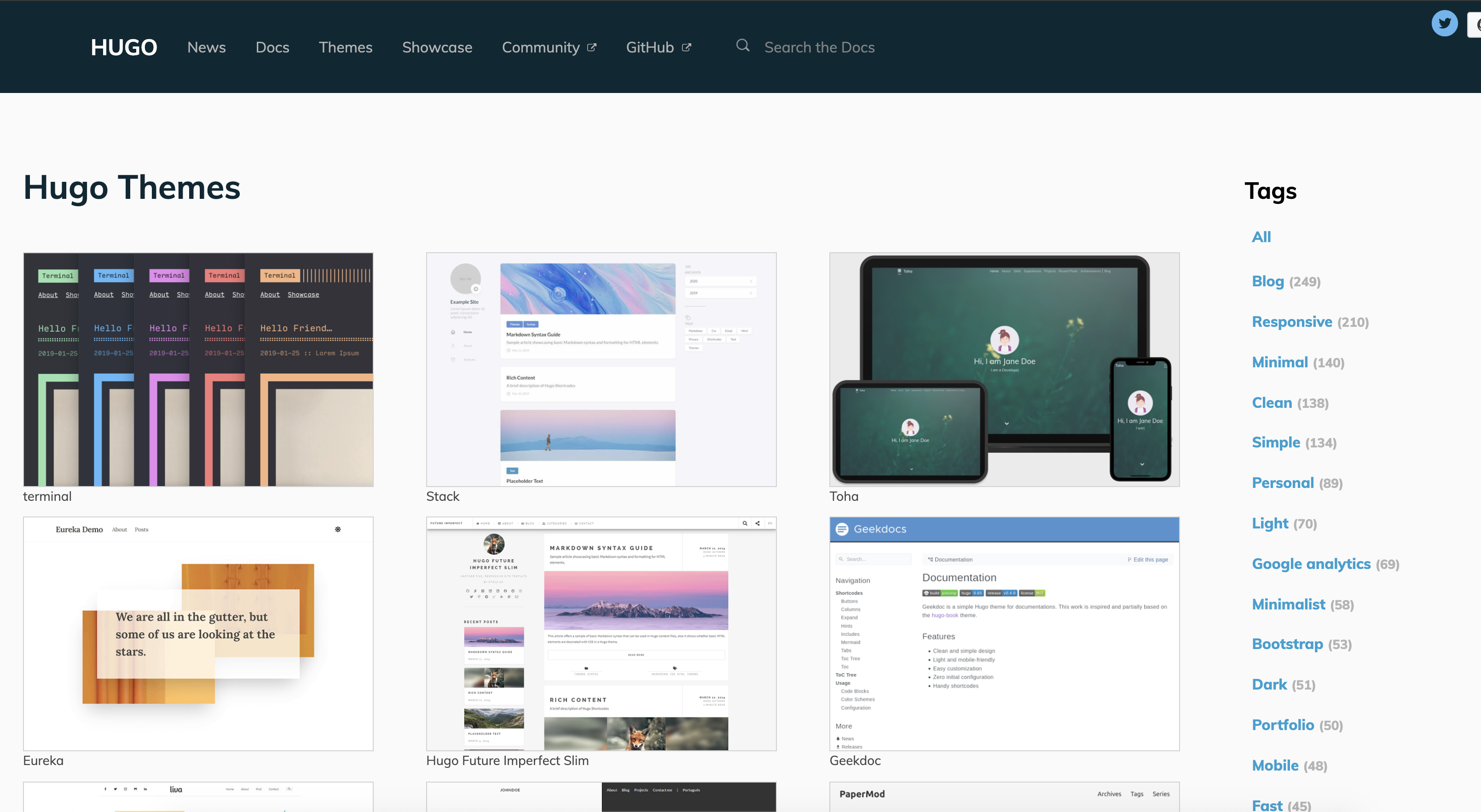
blogdown package, built on the static website generator Hugo: provides support for developing a website from .Rmd files based on Hugo

Benefits of blogdown/Hugo combination over rmarkdown built in generator:

• Hugo is a general-purpose site generator that is highly customizable
• Supports more features, e.g. RSS feeds, metadata especially common in blogs such as categories and tags
• faster to render content
• extended syntax, which means it is highly suitable for technical writing
• Many beautiful themes available

Website with Hugo and blogdown

Developing a website with Hugo and blogdown is not that much more complicated. It uses the following file and folder structure:

• config.toml
• content/
• static/
• themes/
• layouts/

You can read more about this in the blogdown book, Chapter 2

Some example websites using Hugo and blogdown:

• Malcolm Barrett
• Me!
• Andreas Handel
  • See Andreas' tutorial on creating a Hugo Academic theme website in blogdown

Resources

Website development using R Markdown

Useful references for creating websites can be found here:

• R Markdown reference guide
• R Markdown basic website themes

Tutorials on creating a website using R Markdown

• Creating websites in R, Emily C. Zabor
• Nick Strayer & Lucy D'Agostino McGowan

More Resources

More advanced website development using R Markdown

• For more advanced website creation using blogdown and the website generator Hugo see Creating websites with R Markdown.
• Appendix B of the blogdown book presents basic information about websites, such as HTML, CSS, and JavaScript
• A good resource for further information on customizing CSS and JavaScript is w3schools

Making interactive plots shiny and dashboards and hosting on websites

• The Shiny Website
• R Markdown: The Definitive Guide, Chapter 5: Dashboards (Layout, Components, Shiny)

References

This lecture is based on Chapter 10.5: Websites in rmarkdown’s site generator from the book R Markdown: The Definitive Guide, by Yihui Xie, J. J. Allaire, Garrett Grolemund

It pulls also from the tutorial Creating websites in R by Emily C. Zabor